Master Method in Action

Master method is a fundamental technique for determining the complexity of a divide and conquer algorithm. The goal of this post is to show you how to apply the master method while keeping the theoretical details to the bare minimum.

To achieve this, I will introduce a flowchart diagram to guide you in finding the solution.

Divide and Conquer

First, let’s review what the master method is and when to apply it. The master method is a standard technique for computing the complexity of a divide and conquer algorithm.

Complexity measures how many operations an algorithm requires to produce an output, depending on the length of the input. To classify complexity, we use asymptotic notation, which provides a high-level view of time complexity while ignoring unnecessary details.

The divide and conquer technique consists of two steps:

• Divide: Split the original problem into subproblems and solve them individually.
• Conquer: Combine the sub-solutions into a single solution.

This process is recursive: each level receives a subproblem and keeps splitting it until reaching an elementary case, known as the base case.

To represent the time complexity of algorithms, we use recurrence relations. A recurrence relation is an equation that expresses the value of a function in terms of its previous values. The general form is:

\[T(n) = a\text{ }T\left( \frac{n}{b} \right) + f\left(n\right)\]

This equation has two separate components:

• \(a\text{ }T\left( \frac{n}{b} \right)\) represents the process of breaking the problem into subproblems.
• \(f(n)\) represents the process of combining the sub-solutions into a final solution.

The recurrence relation describes how we split the problem into multiple subproblems, while the function \(f(n)\) describes how we combine these subproblems to obtain a solution.

Thus, when you need to compute the complexity the complexity of a divide and conquer algorithm, you are essentially solving a recurrence relation. The master method provides a way to solve specific types of recurrence relations.

Note: The master method determines the complexity of an algorithm, but it does not prove its correctness. To do so, we need other mathematical tools.

Master Method

Given a recurrence of the form:

\[T(n) = a\text{ }T\left( \frac{n}{b} \right) + f(n)\]

the master method defines three different cases for the asymptotic complexity, depending on the relationship between \(f(n)\) and \(\log_{b}{a}\):

• Case 1 \(\begin{align*} \text{ If } f\left( n \right) = \Theta(n^{\log_{b}{a}} ) \text{ then } T(n) = \Theta(n^{\log_{b}{a}} \log{n}) \end{align*}\)

• Case 2 \(\begin{align*} \text{ If } f\left( n \right) = O(n^{\log_{b}{a-\epsilon}}) \text{ for some } \epsilon \gt 0 \text{ then } T(n) = \Theta(n^{\log_{b}{a}}) \end{align*}\)

• Case 3 \(\begin{align*} \text{ If } f\left( n \right) = \Omega(n^{\log_{b}{a+\epsilon}}) \text{, and } \exists N, k < 1 \text{ such that } \forall n\ge N, \end{align*}\) \(f\left( \frac{n}{b} \right)\le k f\left( n \right) \text{, then } T(n) = \Theta(f\left( n \right))\)

This might seem confusing at first, so let’s break it down:

• Our goal is to determine the asymptotic complexity of \(T(n)\), which is given on the right side of each case.
• The complexity function \(T(n)\) is always of the form \(\Theta()\).
• The key idea lies in the relationship between \(n^{\log_{b}{a}}\) and \(f(n)\).
• This relationship is expressed using asymptotic notation.

If the asymptotic relationship between \(n^{\log_{b}{a}}\) and \(f(n)\) fits into one of the three cases above, we can directly determine the asymptotic complexity of \(T(n)\).

The next question is: how do we determine this asymptotic relationship? We can use the limit of the ratio between polynomials.

Limit of Polynomial Ratios for Theta

Given two functions, \(f(n)\) and \(g(n)\), we determine their asymptotic relationship by computing the limit of their ratio. Consider the following case:

\[\text{if} \lim_{x \to \infty } \frac{f(n)}{g(n)}=k \gt 0 \text{ then } f(n) = \Theta(g(n))\]

In simple terms, if the ratio of two polynomial functions approaches a finite, positive constant, then they belong to the same \(\Theta\) complexity class. But why does this matter?

Looking at Case 1 of the master method, the condition requires:

\[f\left( n \right) = \Theta(n^{\log_{b}{a}} )\]

This condition holds if:

\[\lim_{x \to \infty } \frac{f\left( n \right)}{n^{\log_{b}{a}}}= k \gt 0\]

If this limit is positive and finite, we conclude that we are in Case 1 of the master method.

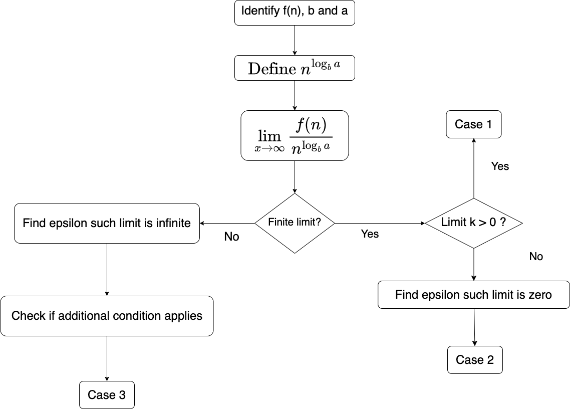
Now, let’s summarize this concept using a flowchart:

Great! Now we understand how to handle the first case. But what about cases 2 and 3? These require a different approach, which we will clarify using another flowchart.

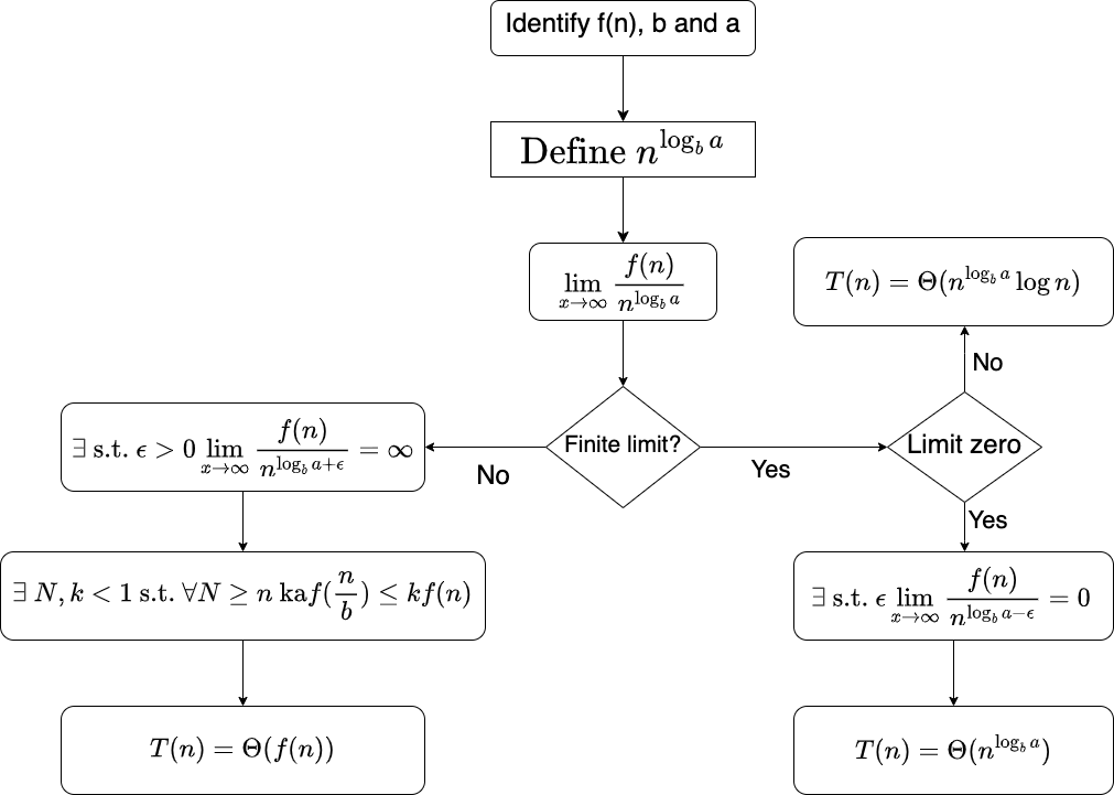
Complete Flowchart

Figure 2 expands on the previous case. First, we check if we have a finite limit, and if it is a positive constant, we are in Case 1. But what if the limit is zero?

This is where the trick comes in. Looking back at Case 2 of the master method, we notice that it is somewhat similar to Case 1—both require a relationship between \(f(n)\) and \(n^{\log_b{a}}\). A full mathematical proof is beyond the scope of this post, but intuitively, a limit of zero is close enough to a positive constant, making it worthwhile to follow a similar reasoning process.

At first, we compute the limit and observe its value. However, here we impose the limit to be zero and look for an \(\epsilon\) that satisfies this condition. In other words, we have flipped the reasoning: previously, we determined the value of the limit from its formulation, but now we manipulate the limit using the Theta notation to obtain the value we need.

Case 3 follows a similar approach. If the limit is infinite, we need to find a Theta value that satisfies the conditions. Additionally, we must verify another condition, known as regularity. However, the core reasoning remains the same.

Now, we can consider the fully formalized flowchart. It follows the same reasoning as before but explicitly lays out all the mathematical steps. If you find it confusing, revisit the simplified version, as they essentially convey the same concepts.

Next, let’s go through some examples to demonstrate how to apply this method.

Note: In the following exercises, we assume that the Master Method can be applied. However, be aware that this is not always the case.

Example: Case 1

Consider the following recurrence:

\[T(n) = 2T\left(\frac{n}{2}\right) + n\]

Using the flowchart, we first isolate the base components: a = 2, b = 2, and f(n) = n. Next we compute \(n^{\log_a{b}} = n^{\log_2{2}} = n\) and take the limit:

\[\lim_{n \to \infty } \frac{f(n)}{ n^{\log_a{b}}} = \lim_{n \to \infty } \frac{n}{ n } = 1\]

Since the limit is positive and finite, we confirm that this falls under Case 1.

Example: Case 2

Consider the recurrence: \(T(n) = 4T\left(\frac{n}{2}\right) + n \log n\)

Following the same steps, we compute \(\log_b{a}\) which is \(n^{\log_2{4}} = n^2\). Next we compute the limit

\[\lim_{n \to \infty} \frac{n \log n}{n^2} = \lim_{n \to \infty} \frac{\log n}{n} = 0\]

However, this time, the limit does not immediately match a known case. Instead of computing the limit, we look for an \(\epsilon\) that satisfies the condition:

\[\exists \epsilon > 0 \text{ such that } \lim_{n \to \infty} \frac{n \log n}{n^{\log_2{4} - \epsilon}} = 0\]

If we simplify the limit we get the following result.

\[\lim_{n \to \infty} \frac{n \log n}{n^{2 - \epsilon}} = 0, \quad \text{if } \epsilon < 1\]

Example: Case 3

Consider the recurrence: \(T(n) = 4T\left(\frac{n}{2}\right) + n^2 \cdot (\log n)^2\)

The \(\log_b{a}\) is the same as before, \(\log_b{a}\) which is \(n^{\log_2{4}} = n^2\). However, if we compute the limit we obtain

\[\lim_{n \to \infty} \frac{n^2 \sqrt{n}}{n^2} = \lim_{n \to \infty} \sqrt{n} = \infty\]

So from the flowchart we know we have to investigate Case 3. First we verify the existence of an epsilon such that

\[\exists \epsilon > 0 \text{ such that } \lim_{n \to \infty} \frac{n^2 \cdot \sqrt{n}}{n^{2 + \epsilon}} = \infty\]

If we simplify the limit we can see that the condition is satisfied if

\[\lim_{n \to \infty} \frac{\sqrt{n}}{n^{\epsilon}} = \infty, \quad \text{if } \epsilon < \frac{1}{2}\]

Finally, we can verify the condition:

\[\exists k > 0 \text{ such that } 4 \left(\frac{n}{2}\right)^2 \sqrt{\frac{n}{2}} \leq k n^2 \sqrt{n}\]

Simplify the element to see that the condition is satisfied with \(k \geq \frac{1}{ \sqrt{2} }\).

Summing Up

In this post, we introduced the master method and demonstrated how to apply it. We used a flowchart to visualize the steps and discussed examples for each case.

By following this approach, you can systematically determine the complexity of divide and conquer algorithms.